In a Neural network, there is a loss function that tells us the performance of the model at the current instant. This loss function is used to train the network such that it can perform better. The loss is taken and we try to minimize it. The lower the loss, the better is performance of the model. The process of optimizing any mathematical expression is called Optimization.

What are optimizers?

Optimizers are algorithms or methods used to change the attributes of the neural network such as weights and learning rate to reduce the losses. Optimizers are used to solve optimization problems by minimizing the function.

There are different types of optimizers (Names are based on the algorithms each implements ):

• Adam

• Gradient descent (with momentum) optimizer (SGD)

• RMSprop

• AdaDelta

• Adaptive Gradient (AdaGrad)

• Nadam

• Adamax

• "Follow The Regularized Leader" (FTRL)

To know more about optimizers refer to the documentation from Keras.

In this Blog, I will be comparing the different optimizers using the MNIST dataset and comparing the results.

Let's start with the imports

import tensorflow as tf
from matplotlib import pyplot as plt

Loading MNIST dataset

# Load the dataset and repshape the data
(trainX, trainY), (testX, testY) = tf.keras.datasets.mnist.load_data()
# X represets images and Y represents image labels

trainX = tf.keras.utils.normalize(trainX, axis=1)
testX = tf.keras.utils.normalize(testX, axis=1)

# Reshape the data to 4D tensor format (batch_size, height, width, channels)
trainX = trainX.reshape(trainX.shape[0], 28, 28, 1).astype('float32')
testX = testX.reshape(testX.shape[0], 28, 28, 1).astype('float32')

# Convert labels to one-hot encoding
trainY = tf.keras.utils.to_categorical(trainY, 10)
testY = tf.keras.utils.to_categorical(testY, 10)

Creating the model and evaluation

I will be utilizing a Convolutional Neural Network (CNN) for this task. CNNs are particularly well-suited for image-related tasks, and given that MNIST consists of images of handwritten digits, the inherent ability of CNNs to capture spatial hierarchies makes them an effective choice for achieving accurate digit classification and for testing out optimizers.

Creating the model

def create_models(optimizer):
    model = tf.keras.models.Sequential()

    #convolution and pooling layers
    model.add(tf.keras.layers.Conv2D(32,(3,3), activation = 'relu', input_shape = (28,28,1)))

    model.add(tf.keras.layers.MaxPooling2D((2,2)))
    model.add(tf.keras.layers.Conv2D(64,(3,3), activation = 'relu'))
    model.add(tf.keras.layers.MaxPooling2D((2,2)))
    model.add(tf.keras.layers.Conv2D(64,(3,3), activation = 'relu'))

    model.add(tf.keras.layers.Flatten())

    # Dense layers for classification
    model.add(tf.keras.layers.Dense(128, activation='relu'))
    model.add(tf.keras.layers.Dense(10, activation='softmax'))

    #Compile model
    model.compile (optimizer = optimizer, loss = 'categorical_crossentropy' , metrics =['accuracy'])

Evaluation of the model

def evaluate_model(optimizer, model):
  val_loss, val_acc = model.evaluate(testX,testY)
  print("OPTIMIZER USED : ",optimizer, "\n")
  print("loss --> ", val_loss, "\naccuracy -->",val_acc)

• There is a detailed blog in which I have done digit classification on MNIST using CNN. You can check it out here: BLOG

• so now we can move on to the main topic of this blog

Comparing Optimizers

I have set the epoch to 5, for ease

#Optimizers i will be using.
optimizers = ['adam', 'sgd', 'rmsprop', 'adadelta', 'adagrad','adamax','nadam','ftrl']
#Train the models with different optimizers

for optimizer in optimizers :
  model = create_models(optimizer)
  history  = model.fit(trainX, trainY, epochs=5, batch_size=64, validation_split=0.2)

• In this, I have added optimizers in a list named optimizers

• The for-loop iterates over the optimizers

• The model is then trained using the fit method. It undergoes five training epochs (epochs=5) with a batch size of 64 (batch_size=64). The training process includes the MNIST training data (trainX and trainY), and 20% of the data is used as a validation set (validation_split=0.2) to monitor the model's performance during training.

Now we will add the logic for comparing optimizers and storing the result of training, which will be used for comparison.

import pandas as pd

optimizers = ['adam', 'sgd', 'rmsprop', 'adadelta', 'adagrad','adamax','nadam','ftrl']
optimizer_df = pd.DataFrame(columns=['Optimizer', 'Loss', 'Accuracy'])

for optimizer in optimizers:
    model = create_models(optimizer)

    history = model.fit(trainX, trainY, epochs=5, batch_size=64, validation_split=0.2)

    # Evaluate model
    evaluation_result = evaluate_model(optimizer, model)

    # Check if the evaluation result is not None
    if evaluation_result is not None and len(evaluation_result) == 2:
        loss, accuracy = evaluation_result
        # Append information to the DataFrame
        optimizer_df = optimizer_df.append({'Optimizer': optimizer, 'Loss': loss, 'Accuracy': accuracy}, ignore_index=True)
    else:
        print(f"Warning: Evaluation result for {optimizer} is None")

• The evaluate_model function, passing the optimizer and the trained model. It returns the evaluation results, presumably a tuple containing the loss and accuracy.

• If the evaluation result is valid, it unpacks the tuple into the loss and accuracy variables.

• The information about the optimizer, loss, and accuracy is appended to a DataFrame (optimizer_df). The ignore_index=True parameter ensures that the DataFrame index is renumbered.

Now we can also plot the accuracy. For the following

# Create subplots
fig, (ax1, ax2) = plt.subplots(1, 2, figsize=(12, 4))

# Plot training accuracy
ax1.plot(history.history['accuracy'], label=f'{optimizer}_train', linestyle='--')
ax1.set_title('Training Accuracy')
ax1.set_xlabel('Epochs')
ax1.set_ylabel('Accuracy')
ax1.legend()

# Plot validation accuracy
ax2.plot(history.history['val_accuracy'], label=f'{optimizer}_val')
ax2.set_title('Validation Accuracy')
ax2.set_xlabel('Epochs')
ax2.set_ylabel('Accuracy')
ax2.legend()

as follows. This is the complete function

# optimizers = ['ftrl']
optimizers = ['adam', 'sgd', 'rmsprop', 'adadelta', 'adagrad','adamax','nadam','ftrl']

optimizer_df = pd.DataFrame(columns=['Optimizer', 'Loss', 'Accuracy'])
# Create subplots
fig, (ax1, ax2) = plt.subplots(1, 2, figsize=(12, 4))

for optimizer in optimizers:
    model = create_models(optimizer)
    history = model.fit(trainX, trainY, epochs=5, batch_size=64, validation_split=0.2)

    # Evaluate model
    evaluation_result = evaluate_model(optimizer, model)

    # Check if the evaluation result is not None
    if evaluation_result is not None and len(evaluation_result) == 2:
        loss, accuracy = evaluation_result
        # Append information to the DataFrame
        optimizer_df = optimizer_df.append({'Optimizer': optimizer, 'Loss': loss, 'Accuracy': accuracy}, ignore_index=True)
    else:
        print(f"Warning: Evaluation result for {optimizer} is None or has unexpected format.")

    # Plot training accuracy
    ax1.plot(history.history['accuracy'], label=f'{optimizer}_train', linestyle='--')
    ax1.set_title('Training Accuracy')
    ax1.set_xlabel('Epochs')
    ax1.set_ylabel('Accuracy')
    ax1.legend()

    # Plot validation accuracy
    ax2.plot(history.history['val_accuracy'], label=f'{optimizer}_val')
    ax2.set_title('Validation Accuracy')
    ax2.set_xlabel('Epochs')
    ax2.set_ylabel('Accuracy')
    ax2.legend()

# Display the DataFrame with optimizer information
print(optimizer_df)

# Show the plots
plt.show()

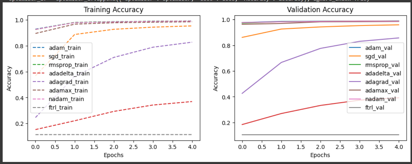
• plt.subplots(1, 2, figsize=(12, 4)) creates a figure (fig) with 1 row and 2 columns of subplots.

• (ax1, ax2) are the axes (subplots) returned by this function. ax1 corresponds to the first subplot, and ax2 corresponds to the second subplot.

• This is used to compare the training and validation accuracy over epochs for different optimizers on side-by-side subplots within the same figure

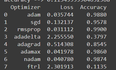
Result

This is the Data for each optimizer :

This is the graph:

You can refer to the implementation in collab

Conclusion

In conclusion, this comparative exploration serves as a compass for navigating the optimization landscape, providing insights into the strengths and trade-offs of various optimizers. The optimal choice may not be universal but rather a dynamic decision influenced by the specific characteristics of the task at hand.

The above-mentioned implementation is just one way of doing it. There can be other efficient ways to implement it. Feel free to send a DM, if you find any mistakes or if it is missing something.