Image classification is one of the most prominent technologies. It is used in powering applications like facial recognition, self-driving cars, and many more. In this blog, I will be sharing an example of Digit image classification, leveraging the power of Convolutional Neural Networks (CNNs). Our journey will revolve around a classic dataset — MNIST, which serves as the perfect playground for understanding the intricate workings of CNNs in the realm of computer vision.

Aim

The MNIST dataset is a collection of 28x28 grayscale images of handwritten digits (0-9), making it an ideal playground for beginners entering the world of computer vision and deep learning. Our goal is to build a CNN that can accurately identify and classify these digits.

Digit Classification using CNN

Key things that I will be doing in this blog

• Dataset preparation

• Model Architecture

• Compilation

• Training and Evaluation

For starters, we will first do the imports we want

import tensorflow as tf
import numpy as np
import random
import matplotlib.pyplot as plt

Dataset Preparation

# Load the dataset and repshape the data
(trainX, trainY), (testX, testY) = tf.keras.datasets.mnist.load_data()

# Normalize the pixel values
trainX = tf.keras.utils.normalize(trainX, axis=1)
testX = tf.keras.utils.normalize(testX, axis=1)

# Reshape the data to 4D tensor format (batch_size, height, width, channels)
trainX = trainX.reshape(trainX.shape[0], 28, 28, 1).astype('float32')
testX = testX.reshape(testX.shape[0], 28, 28, 1).astype('float32')

# Convert labels to one-hot encoding
trainY = tf.keras.utils.to_categorical(trainY, 10)
testY = tf.keras.utils.to_categorical(testY, 10)

• Loads the dataset (X represents images and Y represents image labels)

• Normalize the pixel values,

• Reshape the data into the required 4D Tensor format (Check this docs to know about tensors)

• Convert the labels to one-hot encoding

Model Architecture

model = tf.keras.models.Sequential()
#convolution and pooling layers
model.add(tf.keras.layers.Conv2D(32,(3,3), activation = 'relu', input_shape = (28,28,1)))

model.add(tf.keras.layers.MaxPooling2D((2,2)))
model.add(tf.keras.layers.Conv2D(64,(3,3), activation = 'relu'))
model.add(tf.keras.layers.MaxPooling2D((2,2)))
model.add(tf.keras.layers.Conv2D(64,(3,3), activation = 'relu'))
model.add(tf.keras.layers.Flatten())
# Dense layers for classification
model.add(tf.keras.layers.Dense(128, activation='relu'))

# output layer 
model.add(tf.keras.layers.Dense(10, activation='softmax'))

• Sequential allows us to build a model, layer by layer (by stacking each layer)

• Max pooling layers reduce the spatial dimensions of the representation, helping the network focus on the most important features.

• Flatten layer converts the 2D matrix data to a vector, preparing it for the fully connected layers.

Compilation

model.compile(optimizer= 'adam',
             loss = 'categorical_crossentropy',
             metrics=['accuracy'])

• categorical_crossentropy as a loss function because we are classifying multiclass problems and also one-hot encoded data

• adam because it is one of the popular optimization algorithms, known for its adaptive learning rates and efficient handling of sparse gradients. (It determines how the model's weights are updated during training to minimize the loss function)

Training

model.fit(trainX, trainY, epochs=5, batch_size=64, validation_split=0.2)

Valuation

val_loss, val_acc = model.evaluate(testX,testY)
print("loss --> ", val_loss, "\naccuracy -->",val_acc)

Plotting Predictions

# Functions for Plotting the predictions 
def grpah_plot(indices):
    # Randomly select 4 indices from the test data
  fig, axes = plt.subplots(1, 5, figsize=(15, 5))  # Adjusted figure size
  for i, index in enumerate(indices):
      reshaped_image = testX[index].reshape(28, 28)  # Reshape the image to (28, 28)
      axes[i].imshow(reshaped_image, cmap='gray')
      axes[i].axis('off')
      axes[i].set_title(f'True: {np.argmax(testY[index])}\nPred: {np.argmax(pred[index])}')  
      # Set titles with true and predicted labels
  plt.show()

#Function for scatter plot
def scatter_plot (indices) :
  random_indices = random.sample(range(len(testX)), 50)
  # Get true labels and predicted labels for the selected indices
  true_labels = np.argmax(testY[indices], axis=1)
  predicted_labels = np.argmax(pred[indices], axis=1)

  # Create a scatter plot
  plt.figure(figsize=(10, 6))
  plt.scatter(range(len(indices)), true_labels, color='blue', label='True Labels', marker='o')
  plt.scatter(range(len(indices)), predicted_labels, color='red', label='Predicted Labels', marker='x')
  plt.xlabel('Sample Index')
  plt.ylabel('Label')
  plt.legend()
  plt.title('True vs. Predicted Labels (Randomly Selected Samples)')
  plt.show()

Graph Plot

• Takes in a list of indices (indices) as input.

• It then iterates through the provided indices, retrieves the corresponding images from the testX dataset, and displays them along with their true and predicted labels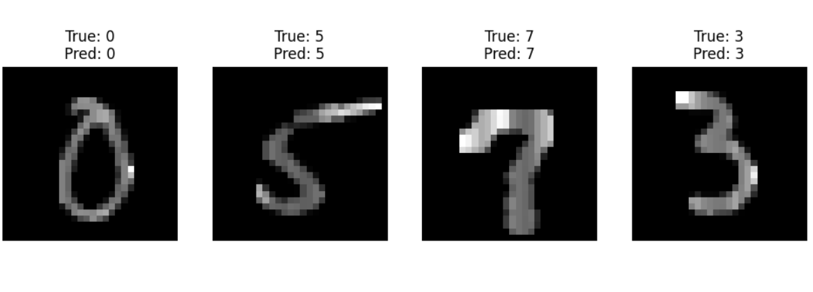

• 

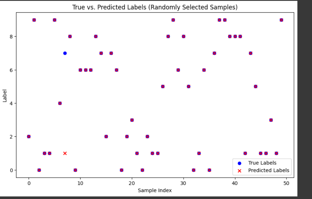
Scatter Plot

• Takes in a list of indices (indices) as input.

• It then retrieves the true labels and predicted labels for the provided indices and creates a scatter plot.

• The scatter plot displays true labels in blue and predicted labels in red, with markers ('o' for true labels, 'x' for predicted labels).

• The x-axis represents the sample indices, and the y-axis represents the label values.

  

Conclusion

Try out the code, if you have any doubts then check this collab file: Collab

In conclusion, the exploration of digit classification on MNIST serves as a stepping stone for tackling more complex image recognition tasks and understanding the inner workings of neural networks.