If you have learned about Neural Networks, then you will be familiar with weight initializations and how crucial it is. Weight initialization, the process of setting the initial values of the weights in a neural network, plays a pivotal role in the network's ability to learn effectively and converge to optimal solutions.

Now, why is this initial setup so important? Well, it's like giving your friend a good starting point. If they start too far away or too close, they might struggle to understand the lessons (data) you're teaching them.

In our neural network world, if we set these initial weights just right, the learning process becomes smoother. The network can grasp patterns and make sense of things quicker. But if we get it wrong, it's like your friend with glasses trying to learn without wearing them – things get (blurry)confusing.

Xavier (Glorot) Initialization

Xavier initialization, also known as Glorot initialization, is specifically designed for networks using sigmoid or hyperbolic tangent (tanh) activation functions.

Benefits of Xavier Initialization:

• Mitigates the vanishing/exploding gradient problem for networks with sigmoid or tanh activations.

• Facilitates stable and efficient training, leading to better convergence.

Kaiming (He) Initialization

Kaiming initialization, also known as He initialization, is tailored for networks using rectified linear units (ReLU) activation functions.

Benefits of Kaiming Initialization:

• Particularly effective for networks employing ReLU activations.

• Addresses the challenges of vanishing gradients and promotes faster convergence.

For more, you can refer to other sources. In this blog I will focus on the execution of the code.

So, now we can start with the imports

Import

import tensorflow as tf
import numpy as np
import matplotlib.pyplot as plt
from tensorflow.keras.models import Sequential
from tensorflow.keras.layers import Flatten, Dense
from tensorflow.keras.utils import to_categorical

Loading the Dataset

cifar10 = tf.keras.datasets.cifar10
(x_train, y_train), (x_test, y_test) = cifar10.load_data()
x_train, x_test = x_train / 255.0, x_test / 255.0

Weight Initialization

Now let's initialize the model sequential and a variable initializer .

Kaiming Weight Initialization

model = Sequential()
initializer = tf.keras.initializers.HeNormal(seed = 0)

#input layer
model.add(Flatten(input_shape=(32, 32, 3)))
# Hidden Layer
model.add(Dense(1024, activation='relu',kernel_initializer=initializer))
model.add(Dense(512, activation='relu',kernel_initializer=initializer))
model.add(Dense(256, activation='relu',kernel_initializer=initializer))

#output layer
model.add(Dense(10, activation='softmax'))

Compiling the model

model.compile(optimizer='adam', loss='sparse_categorical_crossentropy', metrics=['accuracy'])
kaim = model.fit(x_train, y_train, validation_data=(x_test, y_test), epochs=5)

Xavier Weight Initialization

modelX = Sequential()
initializer = tf.keras.initializers.GlorotNormal(seed = 0)

#input layer
modelX.add(Flatten(input_shape=(32, 32, 3)))
# Hidden Layer
modelX.add(Dense(1024, activation='tanh'))
modelX.add(Dense(512, activation='tanh'))
modelX.add(Dense(256, activation='tanh'))

• the default weight initialization for dense layers is Xavier (Glorot) initialization. Since it is designed to work well with sigmoid and hyperbolic tangent (tanh) activation functions.

compiling the model

modelX.compile(optimizer='adam', loss='sparse_categorical_crossentropy', metrics=['accuracy'])
xav = modelX.fit(x_train, y_train, validation_data=(x_test, y_test), epochs=5)

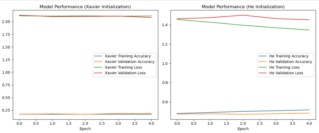
Plotting the Graph

plt.figure(figsize=(12, 5))

# Model using Xavier (Glorot) initialization
plt.subplot(1, 2, 1)
plt.plot(xav.history['accuracy'], label='Xavier Training Accuracy')
plt.plot(xav.history['val_accuracy'], label='Xavier Validation Accuracy')
plt.plot(xav.history['loss'], label='Xavier Training Loss')
plt.plot(xav.history['val_loss'], label='Xavier Validation Loss')
plt.legend()
plt.xlabel('Epoch')
plt.title('Model Performance (Xavier Initialization)')

# Model using He initialization
plt.subplot(1, 2, 2)
plt.plot(kaim.history['accuracy'], label='He Training Accuracy')
plt.plot(kaim.history['val_accuracy'], label='He Validation Accuracy')
plt.plot(kaim.history['loss'], label='He Training Loss')
plt.plot(kaim.history['val_loss'], label='He Validation Loss')
plt.legend()
plt.xlabel('Epoch')
plt.title('Model Performance (He Initialization)')

plt.tight_layout()
plt.show()

This is what we get as the output.

You can also check out the Collab file: Collab

Conclusion

In conclusion, this blog can become a helpful guide for people dealing with the complexities of training neural networks. It provides insights into the small choices that can make a big difference in the success of machine learning models.

The above-mentioned implementation is just one way of doing it. There can be other efficient ways to implement it. Feel free to send a DM, if you find any mistakes or if it is missing something.