In the vast landscape of artificial intelligence, one key challenge is deciphering and understanding sequential data—information that unfolds over time. Whether it's predicting the next word in a sentence, forecasting stock prices, or comprehending the sentiment in a paragraph, the context of what came before is often crucial.

This is where Recurrent Neural Networks (RNNs) step onto the stage. Unlike traditional neural networks, RNNs possess a unique ability to grasp and leverage sequential dependencies. Imagine them as the Sherlock Holmes of the neural network world, adept at deducing patterns and uncovering insights in a story, one chapter at a time.

If you've been reading my blogs, you know I've been documenting the basics of deep learning. In this post, I'll be using RNN to classify the IMDB dataset.

Import

from tensorflow.keras.datasets import imdb
import tensorflow as tf 
import numpy as np

Loading the Dataset

# Set random seed for reproducibility
tf.random.set_seed(42)

# Load IMDB dataset
max_features = 1000
maxLen = 500
batch_size = 32

print("Loading Data ... ")
(train_data, train_labels), (test_data, test_labels) = imdb.load_data(num_words = max_features)

print("Dataset loaded")

• tf.random.set_seed(42) is setting the random seed to ensure reproducibility. In this case, I have set it to 42. Here 42 is used because it is just a convention.

• We are splitting the loaded dataset into labels and data for testing as well as training.

from tensorflow.keras.preprocessing.sequence import pad_sequences

# Pad sequences to have a consistent length
train_data_padded = pad_sequences(train_data, maxlen=maxLen)
test_data_padded = pad_sequences(test_data, maxlen=maxLen)

train_data_np = np.array(train_data_padded)
test_data_np = np.array(test_data_padded)

• The pad_sequences function from TensorFlow's Keras API is used to implement padding.

• This function takes a list of sequences (in this case, train_data and test_data), and it pads or truncates each sequence to ensure a consistent length (maxLen in this case).

• This is crucial when working with text data in natural language processing tasks, where maintaining a uniform sequence length is a common requirement for effective model training and processing.

from tensorflow.keras.utils import to_categorical

# Convert labels to one-hot encoding (if necessary)
train_labels_onehot = to_categorical(train_labels)
test_labels_onehot = to_categorical(test_labels)

• This is used to convert categorical labels into one-hot encoded vectors.

Setting up our RNN model

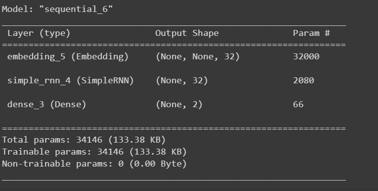
The below code defines a simple RNN-based model for a binary classification task and sets it up for training.

#Building the RNN model
# rom tensorflow.keras.layers import Embedding, SimpleRNN, Dense

model = tf.keras.models.Sequential()
model.add(tf.keras.layers.Embedding(max_features, 32))

model.add(tf.keras.layers.SimpleRNN(32))
model.add(tf.keras.layers.Dense(2,activation = 'sigmoid'))

#Compile the Model
model.compile(optimizer = 'adam', loss = 'binary_crossentropy', metrics = ['accuracy'])
model.summary()

# Train the model
history = model.fit(train_data_padded, train_labels_onehot, epochs=5, batch_size=batch_size, validation_split=0.2)

Result

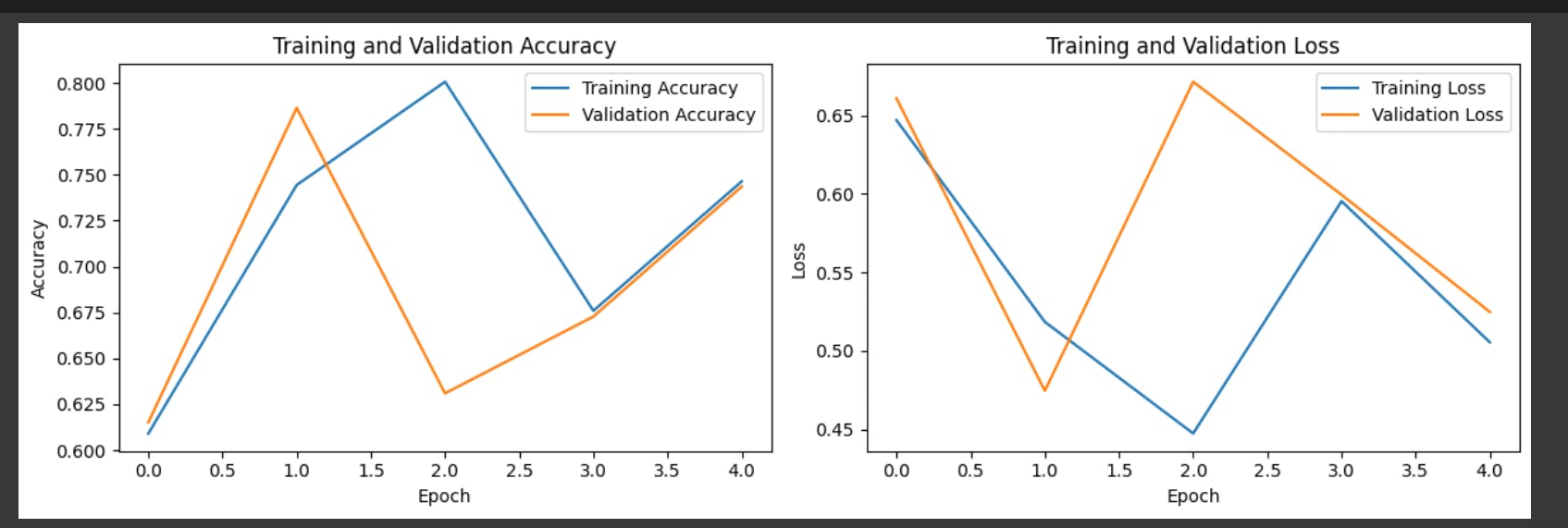
The above is a depiction of the results that we got after training the simple RNN model. I have illustrated the results using a Graph plot and

Graph Plot

import matplotlib.pyplot as plt
# Plot accuracy and validation accuracy
plt.figure(figsize=(12, 4))
plt.subplot(1, 2, 1)
plt.plot(history.history['accuracy'], label='Training Accuracy')
plt.plot(history.history['val_accuracy'], label='Validation Accuracy')
plt.title('Training and Validation Accuracy')
plt.xlabel('Epoch')
plt.ylabel('Accuracy')
plt.legend()

# Plot loss and validation loss
plt.subplot(1, 2, 2)
plt.plot(history.history['loss'], label='Training Loss')
plt.plot(history.history['val_loss'], label='Validation Loss')
plt.title('Training and Validation Loss')
plt.xlabel('Epoch')
plt.ylabel('Loss')
plt.legend()

# Adjust layout and show plots
plt.tight_layout()
plt.show()

• The above code uses Matplotlib to create a side-by-side visualization of training and validation metrics (accuracy and loss) over epochs. Let's break down each part of the code.

• 

Text comparison

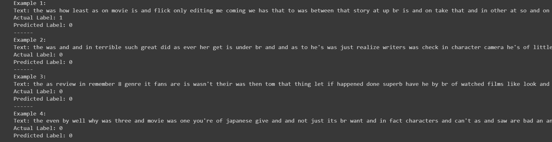
The below code is used to print the comparison between the actual label and the predicted label.

import numpy as np

# Select 4 random indices from the test dataset
random_indices = np.random.choice(len(test_data_padded), size=4, replace=False)

# Get the corresponding sequences and labels
selected_sequences = test_data_padded[random_indices]
selected_labels = test_labels_onehot[random_indices]

# Predict the labels using the trained model
predictions = model.predict(selected_sequences)

# Convert predictions to class labels
predicted_labels = np.argmax(predictions, axis=1)

# Function to convert indices back to words (excluding unknown words)
def indices_to_text(indices, word_index):
    reverse_word_index = dict([(value, key) for (key, value) in word_index.items()])
    return ' '.join([reverse_word_index.get(i, '') for i in indices if i in reverse_word_index])

# Convert indices to text for selected sequences
selected_text = [indices_to_text(sequence, imdb.get_word_index()) for sequence in selected_sequences]

# Print actual and predicted responses along with the text
for i, index in enumerate(random_indices):
    print(f"Example {i + 1}:")
    print(f"Text: {selected_text[i]}")
    print(f"Actual Label: {np.argmax(selected_labels[i])}")
    print(f"Predicted Label: {predicted_labels[i]}")
    print("------")

• This is what it looks like :

  

You can get the above code here : collab

Conclusion

In conclusion, this code provides a glimpse into the real-world application of a trained Recurrent Neural Network (RNN) on the IMDb dataset. By randomly selecting four examples from the test dataset, the code demonstrates how the model predicts sentiment labels for specific movie reviews. This approach not only aids in understanding the model's behavior but also facilitates the identification of areas for potential improvement.

The above-mentioned implementation is just one way of doing it. There can be other efficient ways to implement it. Feel free to send a DM, if you find any mistakes or if it is missing something.